keller-strategies

README from GitHub, fetched on 2026-11-04. Source: https://github.com/SimonKreis/keller-strategies

Keller Strategies

An open-source Python engine for backtesting and live-execution of published Tactical Asset Allocation (TAA) strategies, based on the peer-reviewed research of Dr. Wouter Keller, Meb Faber, Gary Antonacci, and others.

The suite implements the Keller canon (HAA, DAA, VAA, BAA, PAA), verified line-by-line against the source papers, plus Antonacci’s dual momentum (GEM) and Faber’s trend-following GTAA. It compares their performance interactively and generates exact monthly rebalancing signals, including leveraged-ETF variants and configurable margin.

It is a research and verification engine, not investment advice. Nothing in it recommends a strategy, a product or a leverage level; see the Disclaimer.

Rebuilt 2026-07-28 after an adversarial audit, which found that execution price, rebalance date, transaction cost, the meaning of a missing price and the meaning of cash were all implied by a single vectorised expression rather than modelled. It now has an explicit execution ledger, coverage guards, honest metrics and run manifests.

Two further audits followed on 2026-07-29 and found what the first had checked around: DAA applied an absolute-momentum filter its paper disclaims three times, and SMA12 averaged twelve prices where Keller defines thirteen. Both moved every published DAA, BAA and PAA number.

Every number in this repository is lower than it was, and that is the point. KNOWN_GAPS.md is the standing list of what this engine still cannot establish. Read it before quoting any figure.

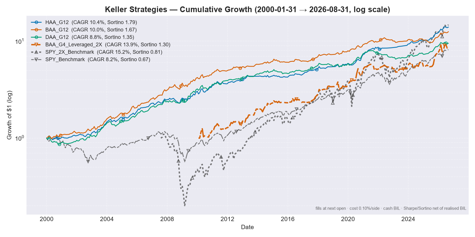
Regenerated 2026-09-23, over the 2000-01 era; each line starts where its products allow. Fills at the next session’s open, 0.10% one-way cost per leg, uninvested weight in BIL, Sharpe and Sortino net of the realised BIL return, wealth curve starting at 1.0. The title states the window that was measured, not the one requested.

Read the leveraged line with the coverage caveat in mind: its products have no bear-market history before 2008, so both 2x lines open years after the others and miss the dot-com bear. See KNOWN_GAPS.md.

Highlights

• 7 strategy families, 35 registered variants. An entry is admitted only if it is a universe its author published, the same on substitute funds, a universe this repo was forced to invent so a leveraged sleeve executes at one uniform multiple, a single-asset control, or a passive benchmark. Sixteen entries went on 2026-07-28, five more on 2026-07-29 and DM_G8_Composite on 2026-09-23 (its mortgage-REIT leg is the one product here with no honest pre-inception donor). One of them, DAA_G3_Leveraged_2X, was restored the same day once the rule that deleted it was restated in the form that chooses a parameter rather than discards a variant. Every row of the report carries its own label: faithful / proxy / custom / control / benchmark.
• The leveraged variants have their own admission rules, written before the backtest, because they are the one part of this repo with no author to defer to. The decisive one: a wrap may change what is HELD, never what decides to DE-RISK. VAA and PAA protect by counting breadth over their own offensive universe, so restricting that universe for LETF execution rewrites the protection rule instead of just narrowing the portfolio; their leveraged variants were deleted, and not because they performed badly. HAA gained one the same day, on the same rule. See LEVERAGE.md §8.
• Desktop dashboard (NiceGUI): backtests and live whole-share order sizing across multiple broker accounts, in a native window. Double-click run_dashboard.bat on Windows, no code required.
• Personal settings stay private: account balances, strategy picks and every user knob live in a gitignored user_config.json, never in the code.
• Leveraged-ETF execution: a faithful “wrap pattern” runs the canonical signal on 1x assets and maps the offensive sleeve to real leveraged ETFs (e.g. SPY → UPRO), holding the defensive sleeve at 1x. Only universes that execute at a uniform multiple are admissible, and the mapper enforces it at construction.
• A single external data source, and a second opinion about it. The engine reads Yahoo Finance for every traded price: no FRED, no macro series, no second provider in the signal path. The one exception is a history donor: the LBMA gold fixing, fetched once to extend GLD before its 2004 inception, which never prices a traded bar. Since 2026-09-01 tools/vendor_crosscheck.py reads a different vendor for verification only: no engine path imports it, and it lives outside tests/ so the suite stays network-free. That tool exists because the price cache was found holding two dividend-adjustment vintages spliced together, invisible to every test in the suite: they all read frozen fixtures, so a data layer wrong in a self-consistent way could not be seen. See KNOWN_GAPS.md §2.
• An explicit execution model: fills at the session after the signal, one-way cost charged per leg on the notional actually traded, positions that drift between rebalances, uninvested weight in a real cash asset, and margin interest day-counted on the balance actually drawn. None of it implied; all of it configurable.
• The engine refuses rather than approximates: a month whose weights do not sum to 1, or that holds a ticker with no price, raises instead of being recorded as a 0% return. A strategy is never measured over years its own products did not exist: the window is trimmed and the binding ticker is named.
• Reports that argue against themselves: a regime panel showing behaviour in nine named drawdowns (n/a where coverage is missing, never a number), the expected best-of-N under the null next to the observed best, and the rank correlation of the leaderboard between disjoint sub-periods. It comes out near zero, and the report says so.
• There is no date picker, and that is the feature: a window you choose is a result you chose. The engine runs a fixed era (2000-01 → the last complete month: every published strategy is measurable from 2000-01, through the dot-com bear and the GFC, because the ETFs’ pre-inception years are carried on older index mutual funds and published indices, each admitted by measurement and flagged as constructed; see KNOWN_GAPS.md §2) and reports every strategy across four pre-registered partitions of it: the NBER business cycle, the S&P 500 bull/bear cycle, the FOMC rate cycle, and BLS CPI inflation regimes. The segments tile the era with no gap and no overlap (a test compounds them back to the era’s own return), and every panel is measured over each strategy’s full history, so no run can shorten a regime. An n/a means the assets did not exist, never “you asked for a shorter window”. The ranked table uses one window shared by every row, derived from the data as the latest inception among the strategies compared, with every binding one named. Ties are the normal case, so naming just one made the report’s own “drop it to lengthen the window” advice false. Since 2026-07-29 entries nobody published (custom) are not allowed to set that window at all: four leveraged G4 wraps were costing all 25 then-registered rows nineteen months and hiding 2008 from the headline drawdown column. Nor is anything holding a leveraged product, whatever its fidelity label: every LETF launched 2006 or later, so a levered benchmark labelled faithful (100% UPRO has no rule to be unfaithful to) would have re-introduced the same defect through the label rather than the role. Both exclusions are in main.may_set_ranked_window. Excluded entries are still measured, in a separate block, over their own window.
• Three answers to “which window?”, because there is no free one: the ranked table gives ONE window to the entries that reach it and measures late arrivals in a clearly separated block; RANKED_WINDOW_POLICY='all' forces one window over everything at the cost of the 2007-2009 bear, the most discriminating stretch in the record; and the dashboard’s common-window comparison intersects the months of whatever you have ticked and re-measures every entry on them, naming the entry that binds so you can untick it. Best for a two- or three-way question, worst for a large selection.
• A leaderboard per regime, not just a matrix. Under the four partition tables, each segment gets its own small ranked table: who actually led the GFC, the COVID crash, the 2022 bear. It inherits the ranked table’s one rule (every row spans the same months), so a strategy that entered a segment late is listed with what it covered and is not ranked. Arriving after the crash shows the recovery without the fall, and ranking that would rebuild date-selection bias inside the very panel built to remove it. The dashboard renders the same thing as nested expansion panels.
• UPI (Ulcer Performance Index): Keller’s own primary ranking metric, (CAGR − rf) / Ulcer Index, alongside CAGR / MaxDD / Sharpe / Sortino / Volatility.
• Provenance on every artefact: each saved report carries a *.manifest.json with the commit, the data hash, the resolved config, and the window actually measured.
• Deterministic test suite with EXTERNAL anchors: momentum checked against a closed form derived in the test file, strategy baskets against arithmetic done by hand, cost against the paper’s stated one-way rate, and a golden master that fails on purpose whenever a fix moves a number.
• Every strategy checked against its own paper’s rule: tests/test_paper_rules.py re-derives each family’s selection rule from hand-built panels, independently of the code. It exists because two Keller-compliance defects survived two audits and 131 self-consistency tests: DAA applied an absolute-momentum filter its paper disclaims three times, and SMA12 averaged twelve prices where Keller defines thirteen. Both moved every published DAA, BAA and PAA number. See KNOWN_GAPS.md §7.
• Every fidelity claim carries a citation. faithful / proxy / custom is no longer a bare string: each entry names the paper, section or figure behind it, and a test asserts all 35 have one. Four labels have been found wrong so far, all four in the under-claiming direction, so since 2026-07-30 every key’s (fidelity, paper, section) is also pinned in tests/test_paper_rules.py::TestFidelityAgainstSource, where a wrong label fails CI instead of waiting for someone to re-read a PDF.

Desktop Dashboard

python app.py        # native desktop window (or your browser as fallback)

On Windows you can simply double-click run_dashboard.bat: the first run sets up the environment automatically, later runs start instantly.

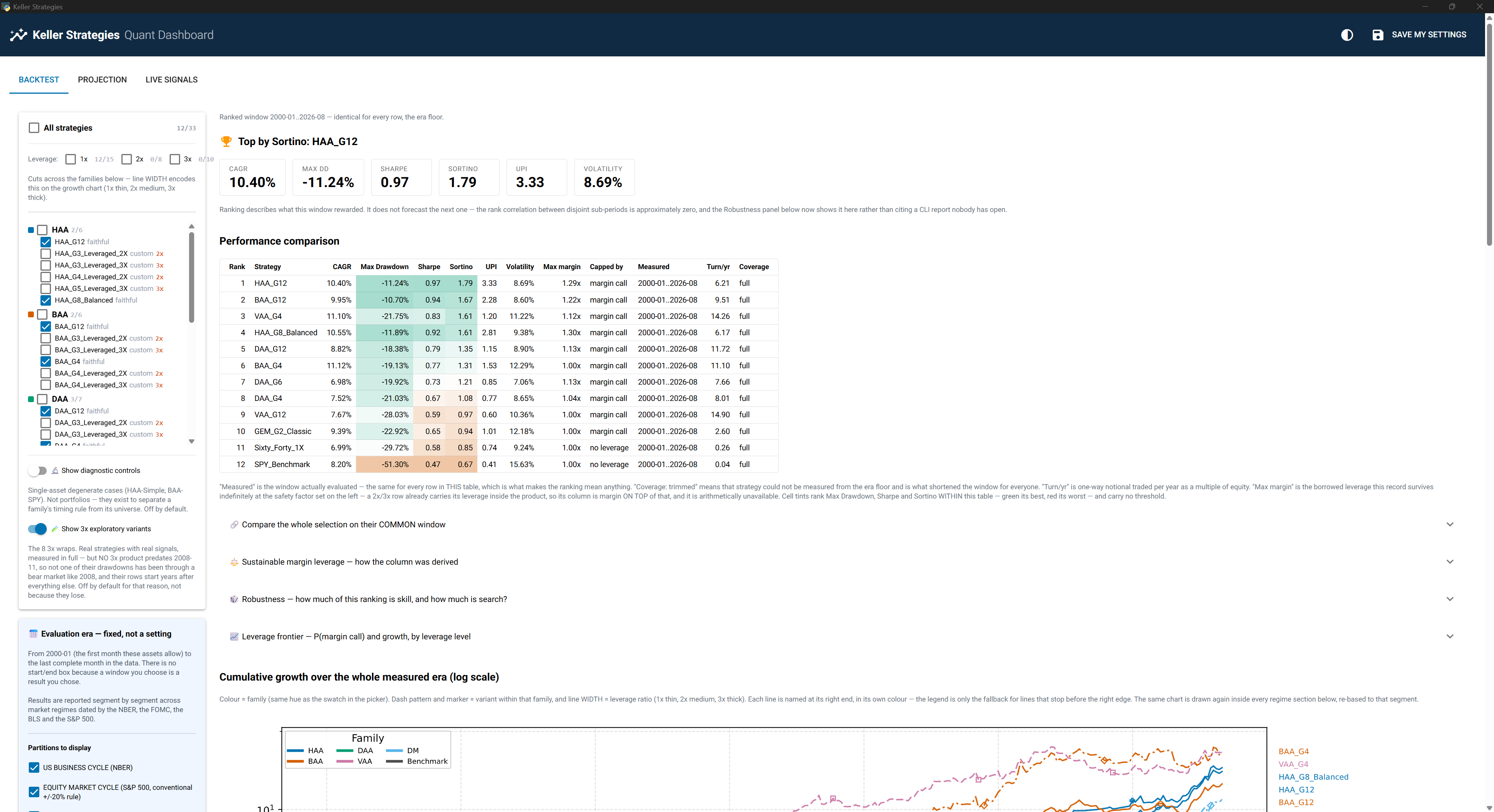
• Backtest tab: set margin leverage, borrowing cost and transaction cost, and get a ranked metrics table (CAGR, Max Drawdown, Sharpe, Sortino, UPI, Volatility) that also shows the window actually measured, realised turnover, and any coverage trim, plus one expandable table per market regime (NBER / S&P 500 / FOMC / CPI), a log-scale growth chart and each strategy’s latest target allocation. There are no start and end date boxes: the era is fixed. Numbers are right-aligned, and Max Drawdown, Sharpe and Sortino are tinted green-to-red within the table: a relative reading, never a threshold.
• The strategy picker is a checklist, ticked by default: every strategy runs unless you untick it, with a master switch and one box per family. It saves what you turned off (EXCLUDED_STRATEGIES), so a variant added to the registry later appears on its own instead of being frozen out by a list written months ago. The two single-asset controls are hidden behind a switch: they are diagnostics for splitting a family’s record into its timing rule and its universe, not portfolios to hold.
• The growth chart encodes three ways at once: colour by family, dash pattern and marker by variant within it, and every line named at its own right-hand end in its own colour. Twenty-odd lines drawn from one continuous colormap were not distinguishable; the legend is now reduced to what the labels cannot say, which is what the hues mean.
• The chart is drawn once per period section, not once per run: the whole era at the top, and again inside every regime segment, re-based to 1.0 at that segment’s start and rendered the first time you open it. “What did this return in the GFC” was already a number; now the path is there too, at a scale where the GFC is not four inches wide. The ADVERSE bucket gets one as well, on an ordinal axis, because those months are not contiguous and a date axis would draw straight lines across the good years between them.
• A Max margin column, and the cap that produced it: how much borrowed leverage each record survives indefinitely, from common/margin_sizing.py. It needs no data from your broker: the credit-line cap reports itself unbounded rather than guessing, the borrow rate was already a knob, and the maintenance requirement comes from a stated convention (30% base, times the fund’s own multiple for a leveraged product). Two columns rather than one, because 1.00x from the Kelly gate (“borrowed money would have reduced growth”) and 1.00x from margin survival (“the broker would have closed you out”) are opposite findings that print the same number.
• A robustness panel that argues against the table above it: three measurements, folded away and computed only when opened. The selection context and rank stability figures the CLI has printed for months and the dashboard merely cited (“the rank correlation between disjoint sub-periods is approximately zero”, pointing at a report nobody had open). PBO, the probability of backtest overfitting, by combinatorially symmetric cross-validation over all 12 870 equal splits of the shared window: 45.5%, with the in-sample crown going to HAA_G12 in only 38.9% of them. And the leaderboard rebuilt on 2 000 resampled histories, so “rank 1” can be read next to “top three in 76.0% of alternative histories”: different claims, now on the same screen. Both measurements also run pooled by family and by de-risking mechanism, because a family whose every variant scores well is harder to explain as luck than one lucky variant. Since the era reached back to 2000, pooling by family no longer helps (45.5% → 50.6%), and only pooling by mechanism does (38.0%); the HAA family is top-3 in 79.0% of alternative histories. Every figure is net of the run’s own realised risk-free rate (the same rate the leaderboard nets), and the section prints the rate it used. None of it forecasts: a bootstrap draws from the distribution it is given, and if these twenty-six years were generous to US assets then so is every resampled path.
• A leverage frontier, cross-checking the sizing from an independent direction: the same resampled histories walked month by month at every constant leverage level from 1.0x to 3.0x, under the ledger’s own monthly-reset policy and each entry’s own maintenance requirement. Three curves per strategy (P(margin call), median CAGR, 5th-percentile CAGR), drawn as two stacked panels (never a dual axis), with the Max margin advice marked on them and its P(call) evaluated on the paths. The closed-form cap and the path walk share the maintenance requirement and the borrow rate and nothing else; measured, they bracket the same band from opposite sides: advice at 1.0–1.3x, month-end calls material only near 2.0x, the gap being exactly the intraperiod factor monthly paths cannot see. The Kelly column is the f that maximises median CAGR across the resampled histories, ruin included.
• Projection tab: give each broker account a kind (registered or not, as common/projection.py defines them), a monthly effort and your tax rates, and get the P10 / median / P90 after-tax value over your horizon, beside a benchmark, a savings account and the money you put in. The return is the strategy’s haircut Sharpe times its volatility, never its CAGR, and the assumptions are printed above the chart. The same computation as python -m tools.projection.
• Live signals tab: enter your broker accounts (filled in priority order) and the order-sizing knobs, and get exact whole-share orders per account for the current monthly signal, with canary status and remaining cash. The signal is monthly, but quantities are sized at the latest live market quote (with automatic fallback to the month-end close when offline), so orders match what your broker actually charges. An optional price cap (PRICE_CAP_MARGIN_PCT) sizes shares at quote × (1 + X%) and reports the cap per order. Enter it as the limit ceiling on after-hours GTC orders (e.g. IBKR Midprice + cap) and they can never be rejected for insufficient funds.
• Save my settings persists everything to user_config.json (gitignored), which the CLI reads too, so the GUI and main.py always agree. The light/dark button beside it follows your system until you pick one, and the choice is saved with the rest.

Data downloads are cached, so re-runs are fast.

Strategies & Research

Fidelity is claimed per strategy, never in blanket form. See strategy_specs/, where each spec cites the paper and page and lists its deviations, and KNOWN_GAPS.md §5 for the summary. Each paper is linked on SSRN below; the PDFs themselves are not redistributed here (SSRN’s terms allow a personal download, not a public copy); download your own copy from the link.

Family	Strategy	Source paper (SSRN)
HAA	Hybrid Asset Allocation	Keller, 2023
BAA	Bold Asset Allocation	Keller, 2022
DAA	Defensive Asset Allocation	Keller & Keuning, 2018
VAA	Vigilant Asset Allocation	Keller & Keuning, 2017
PAA	Protective Asset Allocation	Keller & Butler, 2016
GTAA	Global Tactical Asset Allocation	Faber, 2006
DM	Dual momentum: GEM, the single-module flagship	Antonacci, Dual Momentum Investing (2014)

The five Keller strategies above were verified line-by-line against their source PDFs by three audits (the third found and fixed two defects the first two had missed) and match the papers, including the exact cash-fraction formula CF = (1/T)·rounddown(bT/B) and PAA’s protection factor n1 = a·N/4.

DM_G8_Composite, Antonacci’s equally-weighted four-module composite from SSRN 2042750, was deleted on 2026-09-23. Not for its rules, which were his and verified against Table 10, but for its history: when the era moved to 2000-01, its mortgage-REIT leg (REM, 2007-05) was the one product in the registry with no admissible donor (the mortgage REITs still listed lost 9% through the GFC where the index lost 52%, because the ones that failed are the ones that vanished), and kept, it alone would have held every other row’s window at 2008-07.

Removed on 2026-07-28: FAA, MAA, EAA, LAA, RAA and CAA. Across eight named drawdown episodes none of them ever outperformed every retained strategy, none implemented its source paper faithfully, and LAA measured ρ = 0.93 against the retained Golden Butterfly benchmark. Rationale and evidence: KNOWN_GAPS.md §6. Their papers remain on SSRN, and their paper-side specs remain in strategy_specs/ (faa.md, maa.md, eaa.md, laa.md, raa.md, caa.md), with mpt.md for the MPT paper that was never implemented.

Detailed per-strategy parameter specs are in strategy_specs/; the TIMELINE.md traces the evolution of TAA from Faber to Keller, and WHY_TAA.md covers the rationale for tactical allocation.

Our take (a preference, not an impartial ranking). We lean toward HAA for structural reasons: one external canary (TIP) rather than a breadth count, a defensive sleeve that chooses between BIL and IEF instead of defaulting to one, and the most recent of Keller’s papers. We favour G12 for asset-class breadth (twelve sleeves across US/ex-US equity, REITs, commodities, gold and three bond tenors), not because it ranks first.

That distinction is deliberate. This README used to claim HAA_G12 had “the family’s best Sharpe and Sortino”, which was wrong twice over: on our own window HAA_G1_Simple scored higher on both, and in Keller’s own Dec-1970 → Dec-2022 results HAA-8 beats HAA-12 on max drawdown (−9.7% vs −10.7%) and Sharpe (1.21 vs 1.19) at an identical 15.9% CAGR.

More generally: do not pick a variant from the ranked table. Every backtest report prints the rank correlation of that table between disjoint sub-periods, and it comes out at approximately zero: the ordering describes what each regime rewarded, it does not forecast the next one. That is what the regime panel underneath it is for. This is a personal bias, not a scientific or impartial recommendation, and not financial advice (see the Disclaimer).

Installation

Requires Python 3.11+.

git clone https://github.com/SimonKreis/keller-strategies.git
cd keller-strategies

python -m venv venv
source venv/bin/activate          # On Windows: venv\Scripts\activate
pip install -r requirements.txt
pip install pywebview             # optional: native desktop window for the GUI

On Windows, double-clicking run_dashboard.bat performs this whole setup on first run.

Usage

Dashboard (recommended)

python app.py            # or double-click run_dashboard.bat on Windows

Personal settings: user_config.json

All user-specific values (broker account balances, strategy picks, dates, leverage, sizing knobs…) live in user_config.json at the project root. The file is gitignored, so your personal data never reaches the repository. Copy user_config.example.json to get started. Every key is optional and falls back to the documented defaults in main.py’s USER DASHBOARD section. The GUI’s Save my settings button writes the same file.

Command line

python main.py                                           # run with your user_config.json (or the dashboard defaults)
python main.py --list                                    # list every available strategy key
python main.py --strategy HAA_G12 HAA_G4_Leveraged_2X    # run specific strategies
python main.py --live                                    # force live-signal mode

Key parameters (defaults in main.py, overridable per key in user_config.json):

# No START_DATE / END_DATE: the era is frozen in common/eras.py and runs to the last
# COMPLETE month in the data. Putting those keys back in user_config.json prints a warning
# and changes nothing.
DATA_START_DATE    = '1998-11-01'   # Derived from the era: 13 months of momentum warm-up before 2000-01
LEVERAGE_FACTOR    = 1.0            # Global MARGIN leverage on active strategies (1.0 = none)
MARGIN_BORROW_RATE = 0.06           # Annual interest charged on the borrowed margin portion
EXECUTION_MODE     = False          # False = backtest, True = live target weights

• Backtest mode computes historical monthly allocations and outputs a performance report (CAGR, Max Drawdown, Sharpe, Sortino, Volatility) plus a log-scale growth chart in backtest_results/.
• Live mode outputs the exact target portfolio weights for the configured date, and translates them into whole-share orders across multiple broker accounts, in the GUI’s Live signals tab or on the CLI. The order-sizing knobs (safety-margin reserve, minimum trade size, and FLUSH_ROUND_UP_BAND_PCT: round the last lot up to deploy idle cash in accounts without fractional shares) are documented in main.py’s USER DASHBOARD and set per user in user_config.json.
• Canadian-listed execution of HAA_G12 (the same decision, bought through Canadian funds in CAD or USD) is a separate driver, python -m tools.ca_orders. It is not a strategy and not in the registry; see EXECUTION_CA.md.
• Savings projection covers what the accounts in BROKER_ACCOUNTS could become with monthly contributions, tax by account type (the kinds common/projection.py defines) and inflation: python -m tools.projection (--demo for the example’s fictional accounts). The return is not the backtest’s CAGR: it is the Sharpe left after the same two haircuts the margin sizing applies, times the strategy’s volatility, resampled from its own record and printed beside a benchmark and a savings account, in CAD and USD at today’s rate. The assumptions print before any number, and every rate is yours to enter. It is an assumption, not a forecast. See KNOWN_GAPS.md §4.

How leverage works

Leverage has two independent, composable sources:

1. Leveraged ETFs (2x/3x): realized through the real price history of products like UPRO/TQQQ/TMF, so their internal financing cost and volatility decay are already reflected. Defensive sleeves are held unleveraged at 1x.
2. Margin (LEVERAGE_FACTOR): borrowed-money leverage on active strategies, with interest on the borrowed portion charged via MARGIN_BORROW_RATE.

A 2x leveraged-ETF strategy run at LEVERAGE_FACTOR = 1.3 therefore reaches ≈ 2.6x effective exposure. See ARCHITECTURE.md for module details.

Margin follows the signal

The two mechanisms are not symmetric, and the difference matters. A leveraged-ETF portfolio de-levers by itself: when the canary flips and the strategy rotates from UPRO into IEF, exposure drops to 1x automatically. Flat margin does not: the loan stays drawn, so the defensive sleeve is bought with borrowed money and the portfolio rides the drawdown levered. Swapping instruments while keeping the same nominal factor silently changes the risk profile.

MARGIN_FOLLOWS_SIGNAL (default true) closes that gap by borrowing only against the offensive sleeve:

effective_leverage = 1 + (LEVERAGE_FACTOR - 1) × offensive_weight

Realised average leverage and its range are reported per strategy so the exposure actually taken is visible rather than assumed. Re-measured 2026-09-23 over 2000-01 → 2026-08, the era, which all three reach on admitted pre-inception donors (KNOWN_GAPS.md §2), so the table now contains the dot-com bear and the whole GFC. Fills at the next open, 0.10%/side, cash in BIL, Sharpe/Sortino net of the BIL series, 6%/yr borrow:

Strategy	Mode	CAGR	MaxDD	Sortino	UPI	Avg lev	Turn/yr
HAA_G12	unlevered 1.0x	10.40%	−11.24%	1.79	3.33	1.00x	6.2
HAA_G12	flat 1.3x	11.54%	−15.48%	1.55	2.46	1.30x	8.1
HAA_G12	signal-following 1.3x	11.66%	−14.99%	1.57	2.54	1.24x	7.6
DAA_G12	unlevered 1.0x	8.82%	−18.38%	1.35	1.15	1.00x	11.7
DAA_G12	flat 1.3x	9.46%	−25.36%	1.14	0.83	1.30x	15.2
DAA_G12	signal-following 1.3x	9.70%	−22.02%	1.20	0.96	1.21x	13.9
BAA_G12	unlevered 1.0x	9.95%	−10.70%	1.67	2.28	1.00x	9.5
BAA_G12	flat 1.3x	10.95%	−18.65%	1.44	1.58	1.30x	12.4
BAA_G12	signal-following 1.3x	11.00%	−14.13%	1.62	2.11	1.13x	10.7

Two separate conclusions, and only the first is about the flag:

1. Signal-following beats flat margin on every metric while borrowing less. That is not alpha: it is the removal of a cost that was buying no exposure, since flat margin pays interest to hold treasuries during exactly the months the signal called for safety.
2. Margin at 1.3x buys CAGR and sells everything else. Against the unlevered baseline it raises return by +0.64 to +1.26 pp but worsens max drawdown, Sortino and UPI in all six levered rows, and lifts turnover by 12-31%. Both conclusions read the same over the earlier 2008-06 window; LEVERAGE.md §5 keeps what moved. Whether that trade is worth taking is a decision about risk appetite, not a decision the backtest makes for you, and note that a margin account can be called intramonth, which this model does not simulate at all (KNOWN_GAPS.md §3).

Set the flag to false to reproduce flat-margin behaviour. Passive benchmarks stay at 1x either way.

Admissible leveraged universes

A leveraged strategy is only admissible if its entire offensive sleeve executes at the same multiple. Mixing ratios (or letting an unmapped asset fall through to 1x) makes effective leverage a function of the monthly signal draw, at which point the backtest no longer describes the portfolio held. Two rules gate every mapping, documented in common/letf_mapper.py:

• Leverage homogeneity: one ratio across the whole offensive sleeve. Canaries and the defensive sleeve are exempt: they are signal-only or held at 1x by design.
• $100M liquidity floor: the binding risk at retail size is issuer closure, not spread. Products below the floor were dropped: EURL, DRN (3x) and UBT, EET, EFO, URE (2x). UCO was dropped separately for tracking WTI crude rather than a broad commodity index.

Universe	Assets	2x	3x
G2	SPY, QQQ	✅	✅
G3	SPY, QQQ, IWM	✅	✅
G4	SPY, QQQ, IWM, GLD	✅	❌ no 3x gold product
G12 (Keller’s full universes)	+ VGK, EWJ, VWO, VNQ, GSG, HYG, LQD	❌	❌

2x wraps are role='strategy'; 3x wraps are role='exploratory': registered, measured and reported in full, but excluded from every selection statistic and barred from setting the ranked window. Every 3X twin measured ρ ≈ 0.996-0.999 against its own 2X sibling on shape, which says nothing about depth: 4 of 4 measured pairs show 3x raising CAGR 2.5-5.1 pp while worsening Sortino and UPI and deepening drawdown 13-22 pp. And no 3x product predates 2008-11, so none has bear-market history. This yields 15 leveraged variants (seven 2x, eight 3x) across DAA, BAA, HAA and DM, beside three levered benchmarks. VAA and PAA admit no wrap at all (their protection is a breadth count over the very universe a wrap must restrict; see strategies/vaa.py and strategies/paa.py).

Testing

python -m unittest discover -s tests

Deterministic and network-free. Four categories, and the last two are the ones that matter:

1. Guards. What the engine must REFUSE: an incomplete month, a window predating a strategy’s own products, weights that do not sum to 1, a held ticker with no price, a data gap longer than five trading days, a canary reading bullish on missing data, a regime segmentation that leaves a gap or an overlap in the era, and a price panel carrying more than one dividend-adjustment vintage.
2. Golden master. 8 strategies × 6 metrics pinned over a frozen daily fixture. If a change moves a number this fails on purpose; regenerate it in the same commit, with the reason.
3. External anchors. Comparisons against things the code did not produce: 13612U checked against a closed form written out in the test, HAA’s selection and substitution rules against baskets worked out by hand, Keller’s stated 0.1% one-way cost as arithmetic, and the HAA paper’s published result shape as a sanity band.
4. Paper rules. Each family’s selection rule re-derived from hand-built panels and compared against what its paper actually states. This is the category a golden master cannot replace: a golden master says a number moved, never which rule is right.

The last two exist because of what the audits found. Before 2026-07-28 all 55 tests asserted f(x) == f(x), and every one of them passed against an engine with four critical defects; two further Keller-compliance defects then survived two audits and 131 self-consistency tests. A test that only compares the code to itself adds coverage but no assurance, and, as 2026-09-01 showed, a suite that only reads frozen fixtures cannot notice that the live data layer disagrees with its vendor. That is what tools/vendor_crosscheck.py is for.

Tools

Standalone utilities in tools/. None of them is imported by the engine, and none is needed to run a backtest: each is executed directly. Full commands and caveats live in each file’s module docstring.

Tool	What it is for
backtest_driver.py	The safe entry point for any measurement. It reads every parameter off main, then forces EXECUTION_MODE off and drops broker accounts after applying caller overrides, so a measurement cannot reach the live order path by accident. Use it instead of main.py whenever your user_config.json sets EXECUTION_MODE = True.
timing_luck.py	Month-end rebalancing is one draw from twenty equally defensible schedules. This runs all twenty through the same ledger and reports the spread: what turns a headline drawdown into a distribution. The measured figures live in KNOWN_GAPS.md, which is their one home; this table says what the tool does, not what it found.
proxy_fidelity.py	Re-measures every history donor (the mutual funds and indices that carry the era back to 2000) against the ETF it stands in for, and prints the yardstick beside them: how far apart two REAL funds of the same asset class sit. The admission of each donor is recorded in common/data_engine.HISTORY_BACKFILL; this is how anyone checks it rather than takes it on trust. Opens sockets, so it lives here and not in tests/.
emit_facts.py	Regenerates tests/fixtures/run_facts.json, the artefact the documentation tests compare prose against. Run it when a figure the docs quote has legitimately moved, and commit the JSON in the same commit as the change that moved it.
vendor_crosscheck.py	Compares the cached raw closes against a second vendor, monthly returns plus a split sentinel. The source is Nasdaq’s public historical quotes (no key); Stooq, the first source, has gated automated access since 2026-09-01 and stays available as --provider stooq. First full run, 2026-10-04: 35 of 35 tickers compared, 35 agree. unavailable is never counted as agreement.
ca_orders.py	HAA_G12’s current decision as orders in Canadian-listed funds (HAA_G12_CA). Reads the gitignored ca_execution.json, prints the plan and journals it under the gitignored logs/; it never places an order. --demo runs offline on fictional capital. See EXECUTION_CA.md.
ca_execution_gap.py	Measures how far each Canadian fund drifts from the US ETF it stands in for, in USD, all twelve lines of the mapping. The six like-for-like lines are the yardstick: what the Canadian wrapper alone costs. The figures live in EXECUTION_CA.md.
fx_rate.py	The USD/CAD rate the Canadian path uses (typed by hand, else the Bank of Canada’s daily rate, else Yahoo) or an error: there is no default rate.
projection.py	Projects the accounts forward on the strategy’s haircut record (common/projection.py): P10 / median / P90 after tax, nominal and in today’s dollars, against its comparator and a savings account. Reads the PROJECTION block of user_config.json; --demo uses the example’s fictional accounts. Measures through backtest_driver, at leverage 1.0.

Why momentum?

Momentum is an observation of what markets actually do, not a thesis about what they should do. The signal is the price (the compressed sum of all information and positioning), and a trend-following exit provides built-in protection when leadership reverses. Applied at the asset-class level through ETFs, it captures the momentum premium with lower idiosyncratic risk than stock-level approaches, while the canary signals (e.g. VWO/BND) systematically de-risk the portfolio as conditions deteriorate.

Disclaimer

Not financial advice. This software is for educational, research, and informational purposes only. Past performance does not guarantee future results. Use at your own risk.

Contributing

Contributions are welcome. See CONTRIBUTING.md for guidelines on adding strategies or improving the engine.

License

Released under the MIT License. Copyright 2026 Simon Kreis. Contact: Simon Kreis, M. Sc., simon@kreisconsulting.ca.